R绘制多彩的森林图:基于ggplot2

文章目录
点击蓝字 关注我们

上一周,我们介绍了一篇关于R语言绘制森林图(**forest plot)的帖子(来,挑一款你喜欢的森林图**),不知道没有帮助到各位朋友呢?今天给大家带来一个多彩的的森林图,这个森林图前些日子追加在了上一帖子的评论里,应该有朋友已经看到了。今天就该多彩森林图的实现做个简单介绍。
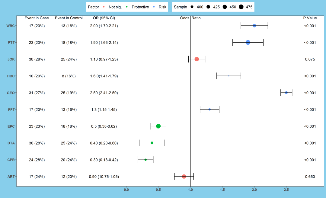
多彩的森林图

需要的R包
该森林图是使用R package:**ggplot2**绘制的,主要用的函数有_ggplot、geom_point、geom_errorbarh、geom_vline、theme和geom_text_。下面我们就一步一步来实现这一多彩森林图吧!
R程序
## 加载程序包
library(ggplot2)
##建立数据集(模拟编造的数据)
dataset <- data.frame(
Varnames = c("ART","WBC","CPR","DTA","EPC","FFT","GEO","HBC","PTT","JOK"),
OR = c(0.9, 2, 0.3, 0.4, 0.5, 1.3, 2.5, 1.6, 1.9, 1.1),
Lower=c(0.75, 1.79, 0.18, 0.2, 0.38, 1.15, 2.41, 1.41, 1.66, 0.97),
Upper=c(1.05, 2.21, 0.42, 0.6, 0.62, 1.45, 2.59, 1.79, 2.14, 1.23),
Factor = c('Not sig.', 'Risk', 'Protective', 'Protective', 'Protective', 'Risk', 'Risk', 'Risk', 'Risk', 'Not sig.'),
Sample=c(450, 420, 390, 400, 470, 390, 400, 388, 480, 460))
#查看数据集
View(dataset)
数据简介
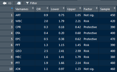
对数据情况做个简单介绍
Varnames:变量名称;
OR:Odds Ratio;
Lower,Upper:95%CI下限及上限;
Factor:影响因素类型;
Sample:样本量。
基于这个数据集,我们开始绘制第一张草图:不同类型变量用不同颜色或形状表示。
画图吧!
##草图
p <- ggplot(dataset, aes(OR, Varnames, col=Factor)) # 不同形状shape= Factor
p + geom_point(size=3.6) +
geom_errorbarh(aes(xmax =Upper, xmin = Lower), height = 0.4) +
scale_x_continuous(limits= c(0.1, 2.6), breaks= seq(0, 2.5, 0.5)) +
geom_vline(aes(xintercept = 1)) +
xlab('Odds Ratio ') + ylab(' ')
# ggsave("forest1.png",dpi = 300,width = 33,height = 20,units = "cm")
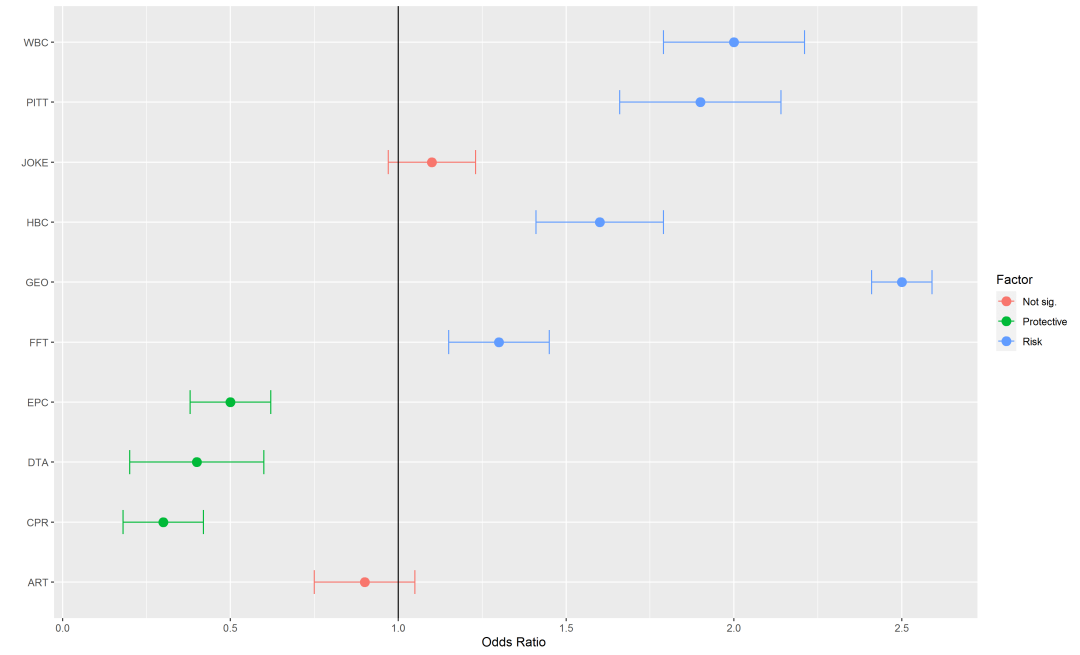

上面已经完成了第一步,下面开始添加文字。
首先通过**data.frame**建立包含P Value和各变量对应的P值的数据框,在通过_geom_text_添加到图中。
## 建立注释内容
annotation <- data.frame(x=c(2.89, 2.89, 2.89, 2.89, 2.89, 2.89, 2.89, 2.89, 2.89, 2.89, 2.89),
y=c(10.47, 10, 9, 8, 7, 6, 5, 4, 3, 2, 1),
label=c('P Value', '<0.001', '<0.001', '0.075','<0.001',
'<0.001', '<0.001', '<0.001', '<0.001', '<0.001', '0.650'))
## 半成品:添加内容
p <- ggplot(dataset, aes(OR, Varnames))
p + geom_point(size=3.6, aes(col=Factor)) +
geom_errorbarh(aes(xmax = Upper, xmin = Lower), height = 0.4)+
geom_vline(aes(xintercept = 1))+theme(legend.position = "top")+
scale_x_continuous(limits=c(0.1, 2.9), breaks = seq(0, 2.5, 0.5))+
geom_text(data=annotation,aes(x=x,y=y,label=label))+
xlab('Odds Ratio ') + ylab(" ")
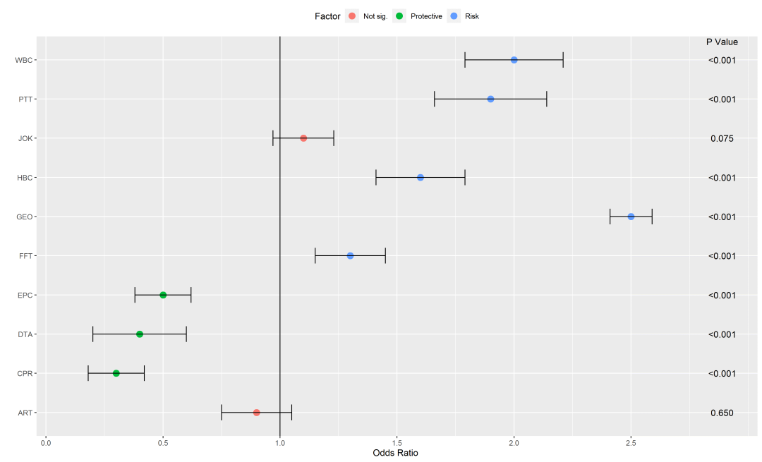
目前是添加了P Value,如果是病例对照研究,我们还可以将病例和对照组暴露人数等数据添加进去。
这里灵活性很大,大家可以根据自己的需要添加相应内容。
建立注释内容
## 建立注释内容(这里也是杜撰的数据)
annotation <- data.frame(
x=c(-1.4, -0.9, -0.35, 1, 2.87, 2.87, 2.87, 2.87, 2.87, 2.87, 2.87, 2.87, 2.87, 2.87, 2.87, -1.4, -0.9, -1.4, -0.9, -1.4, -0.9, -1.4, -0.9, -1.4, -0.9, -1.4, -0.9, -1.4, -0.9, -1.4, -0.9, -1.4, -0.9, -1.4, -0.9, -0.35, -0.35, -0.35, -0.35, -0.35, -0.35, -0.35, -0.35, -0.35, -0.35),
y = c(10.47, 10.47, 10.47, 10.47, 10.47, 10, 9, 8, 7, 6, 5, 4, 3, 2, 1, 10, 10, 9, 9, 8, 8, 7, 7, 6, 6, 5, 5, 4, 4, 3, 3, 2, 2, 1, 1, 10, 9, 8, 7, 6, 5, 4, 3, 2, 1),
label=c('Event in Case', 'Event in Control', 'OR (95% CI)', 'Odds Ratio','P Value', '<0.001', '<0.001', '0.075', '<0.001', '<0.001', '<0.001', '<0.001', '<0.001', '<0.001', '0.650', '17 (20%)',
'13 (16%)', '23 (23%)', '18 (18%)', '30 (28%)', '25 (24%)', '10 (20%)', '8 (16%)', '31 (27%)',
'25 (19%)','17 (20%)','13 (16%)','23 (23%)','18 (18%)','30 (28%)', '25 (24%)', '24 (28%)',
'20 (24%)', '17 (24%)', '12 (20%)', '2.00 (1.79-2.21)', '1.90 (1.66-2.14)', '1.10 (0.97-1.23)',
'1.6 0(1.41-1.79)', '2.50 (2.41-2.59)', '1.3 (1.15-1.45)', '0.5 (0.38-0.62)', '0.40 (0.20-0.60)',
'0.30 (0.18-0.42)', '0.90 (0.75-1.05)'))
成品1:添加注释内容
## 成品1:添加注释内容
p <- ggplot(dataset, aes(OR, Varnames))
p + geom_point(size=3.6, aes(col=Factor)) +
geom_errorbarh(aes(xmax =Upper, xmin = Lower),height = 0.4)+
geom_vline(aes(xintercept=1))+
scale_x_continuous(limits=c(-1.5, 2.87), breaks=seq(0, 2.5, 0.5)) +
xlab(' ') + ylab(" ") + theme_bw() + theme(legend.position ="top") +
theme(panel.grid.major = element_blank(), panel.grid.minor = element_blank(),
plot.background = element_rect(fill ='skyblue', color ='red'),
axis.text=element_text(size=10, face = "bold"),legend.text=element_text(size=11))+
geom_text(data=annotation,aes(x=x,y=y,label=label))
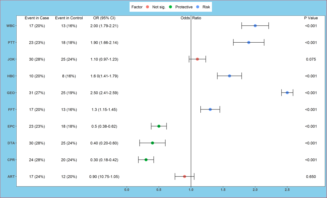
如果是meta分析的森林图,想把样本量大小融入到图里,该如何做呢?
我的做法是用样本量大小去定义圆点的大小。
用样本量定义圆点大小
## 成品2:用样本量定义圆点大小
p + geom_point(aes(size = Sample, col = Factor)) +
geom_errorbarh(aes(xmax = Upper, xmin = Lower), height = 0.4)+
geom_vline(aes(xintercept = 1))+
scale_x_continuous(limits = c(-1.5, 2.87), breaks = seq(0,2.5, 0.5)) +
xlab(' ')+ylab(" ") + theme_bw() + theme(legend.position ="top") +
theme(panel.grid.major = element_blank(), panel.grid.minor = element_blank(),
plot.background = element_rect(fill ='skyblue', color ='red'),
axis.text=element_text(size=10, face = "bold"),legend.text=element_text(size=11))+
geom_text(data=annotation, aes(x=x, y=y, label=label))
大功告成,最后得到的就是生动形象的多彩的森林图啦!

本文分享自微信公众号 - 生信补给站(Bioinfo_R_Python)。
如有侵权,请联系 support@oschina.cn 删除。
本文参与“OSC源创计划”,欢迎正在阅读的你也加入,一起分享。
评论
登录后参与技术讨论,分享你的经验与见解。
登录 / 注册暂无评论