「深度学习」感知机原理与实战(手写数字识别)

文章目录
留个纪念,🕚2022年2月15日上午11时,我的思否创作之路自此开启!🎉🎉🎉
前言
所谓机器学习,在大多数时候都是拿到现有的模型做些简单的修改后就开始“炼丹”,主要工作就是调参,所以江湖人称“调参师”或者“炼丹师”。因此,我想对一些常用的机器学习模型做一些梳理和总结,一来是作为个人的学习笔记,二来是方便各位点进来的朋友复制代码后可以直接开始“炼丹”,争取做到「开箱即用」。
观前提示:这是本人在思否的第一篇文章,水平有限,先在这里给各位大佬赔不是了🙏。
梳理的顺序基本是按照时间来的,大体符合机器学习算法的发展过程,所有模型都会提供其 Pytorch 实现,并简要介绍其原理。本文介绍的是神经网络的鼻祖——感知机。下面开始正文👇
感知机的预备知识
感知机(Perceptron),又称“人工神经元”或“朴素感知机”,是神经网络的基本单元,本文先介绍感知机的基本原理,然后结合具体的分类任务给出感知机模型的 Pytorch 实现。
1.Rosenblatt
Rosenblatt 是神经网络的开山鼻祖,他于 1957 年提出了感知机(Perceptron)的理论;1960 年,他基于硬件结构搭建了一个神经网络。但是,这项成果遭到 Marvin Minksy 和 Seymour Papert 的质疑,使得 Perceptron 沉寂了近 20 年,直到 80 年代 Hinton 发明 BP 算法才使得其成为热门。
2.基本原理
假设输入空间(特征空间)为 \( x\in R^n \) ,输出空间是 \( y\in\{1,-1\} \),则输入空间到输出空间的函数:\( f(x)=sign(wx+b) \) 就称为感知机。其中,w 叫做权值(weight)或权值向量(weight vector),b 叫做偏置(bias),sign 是符号函数:
$$ sign(x)=\begin{cases}1,x\geq0\\-1,x<0\end{cases} $$
给定数据集 \( T=\{(x_1,y_1),(x_2,y_2),\cdots,(x_n,y_n)\} \),则利用感知机进行分类学习的过程等价于求解如下最小化问题:
$$ min L(w,b)=-\sum_{x_i\in M}y_i(wx_i+b_i) $$
其中,M 是误分类点的集合,也就是说感知机是由误分类点驱动的。对于 w 和 b 的更新则是采用随机梯度下降法(SGD):
$$ w^{i+1}=w^i - \eta\frac{\partial L(w,b)}{\partial w}\\ b^{i+1}=b^i - \eta\frac{\partial L(w,b)}{\partial b} $$
其中,\( \eta \) 称为学习率。
单层感知机模型对玩具数据分类
导包
import numpy as np
import matplotlib.pyplot as plt
import torch
%matplotlib inline
加载数据
data = np.genfromtxt('../data/perceptron_toydata.txt', delimiter='\t')
X, y = data[:, :2], data[:, 2]
y = y.astype(np.int)

print('Class label counts:', np.bincount(y))
print('X.shape:', X.shape)
print('y.shape:', y.shape)
输出如下👇
Class label counts: [50 50]
X.shape: (100, 2)
y.shape: (100,)
打乱数据并随机划分训练集和测试集
shuffle_idx = np.arange(y.shape[0])
shuffle_rng = np.random.RandomState(123) #定义一个随机数种子,实现每次代码执行生成的随机数集都相同
shuffle_rng.shuffle(shuffle_idx)
X, y = X[shuffle_idx], y[shuffle_idx]
X_train, X_test = X[shuffle_idx[:70]], X[shuffle_idx[70:]]
y_train, y_test = y[shuffle_idx[:70]], y[shuffle_idx[70:]]对数据进行Z-Score标准化,标准化后的数据均值为0,方差为1,标准化后特征数据的分布没有发生改变。
线性模型一般情况下都需要做数据归一化/标准化处理,如KNN(K近邻)、K-means聚类、感知机和SVM。
决策树、基于决策树的Boosting和Bagging等集成学习模型对于特征取值大小并不敏感,如随机森林、XGBoost、LightGBM等树模型,以及朴素贝叶斯,这些模型一般不需要做数据归一化/标准化处理。
# Normalize (mean zero, unit variance)
mu, sigma = X_train.mean(axis=0), X_train.std(axis=0)
X_train = (X_train - mu) / sigma
X_test = (X_test - mu) / sigma
数据散点图👇,可以明显看出分为两类。
plt.scatter(X_train[y_train==0, 0], X_train[y_train==0, 1], label='class 0', marker='o')
plt.scatter(X_train[y_train==1, 0], X_train[y_train==1, 1], label='class 1', marker='s')
plt.xlabel('feature 1')
plt.ylabel('feature 2')
plt.legend()
plt.show()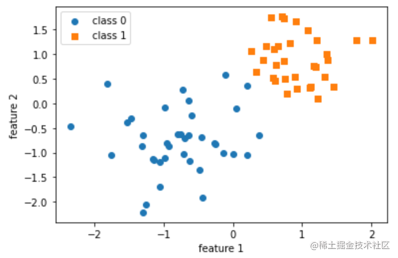
- 模型定义
device = torch.device("cuda:0" if torch.cuda.is_available() else "cpu")


def custom_where(cond, x_1, x_2):
    return (cond * x_1) + ((~cond) * x_2)


class Perceptron():
    def __init__(self, num_features):
        self.num_features = num_features
        self.weights = torch.zeros(num_features, 1,
                                   dtype=torch.float32, device=device)
        self.bias = torch.zeros(1, dtype=torch.float32, device=device)

    def forward(self, x):
        linear = torch.add(torch.mm(x, self.weights), self.bias)
        predictions = custom_where(linear > 0., 1, 0).float()
        return predictions

    def backward(self, x, y):
        predictions = self.forward(x)
        errors = y - predictions
        return errors

    def train(self, x, y, epochs):
        for e in range(epochs):

            for i in range(y.size()[0]):
                # use view because backward expects a matrix (i.e., 2D tensor)
                errors = self.backward(x[i].view(1, self.num_features), y[i]).view(-1)
                self.weights += (errors * x[i]).view(self.num_features, 1)
                self.bias += errors

    def evaluate(self, x, y):
        predictions = self.forward(x).view(-1)
        accuracy = torch.sum(predictions == y).float() / y.size()[0]
return accuracy- 模型训练
ppn = Perceptron(num_features=2)

X_train_tensor = torch.tensor(X_train, dtype=torch.float32, device=device)
y_train_tensor = torch.tensor(y_train, dtype=torch.float32, device=device)

ppn.train(X_train_tensor, y_train_tensor, epochs=10)

print('Model parameters:')
print('Weights: %s' % ppn.weights)
print('Bias: %s' % ppn.bias)
输出如下👇
Model parameters:
Weights: tensor([[1.2734], [1.3464]])
Bias: tensor([-1.])
- 模型评估
X_test_tensor = torch.tensor(X_test, dtype=torch.float32, device=device)
y_test_tensor = torch.tensor(y_test, dtype=torch.float32, device=device)

test_acc = ppn.evaluate(X_test_tensor, y_test_tensor)
print('Test set accuracy: %.2f%%' % (test_acc*100))
输出如下👇
Test set accuracy: 93.33%
效果图
w, b = ppn.weights, ppn.bias

x_min = -2
y_min = ( (-(w[0] * x_min) - b[0])
          / w[1] )

x_max = 2
y_max = ( (-(w[0] * x_max) - b[0])
          / w[1] )


fig, ax = plt.subplots(1, 2, sharex=True, figsize=(7, 3))

ax[0].plot([x_min, x_max], [y_min, y_max])
ax[1].plot([x_min, x_max], [y_min, y_max])

ax[0].scatter(X_train[y_train==0, 0], X_train[y_train==0, 1], label='class 0', marker='o')
ax[0].scatter(X_train[y_train==1, 0], X_train[y_train==1, 1], label='class 1', marker='s')

ax[1].scatter(X_test[y_test==0, 0], X_test[y_test==0, 1], label='class 0', marker='o')
ax[1].scatter(X_test[y_test==1, 0], X_test[y_test==1, 1], label='class 1', marker='s')

ax[1].legend(loc='upper left')
plt.show()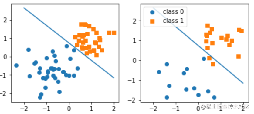
多层感知机模型 & 手写数字识别
导包
import time
import numpy as np
from torchvision import datasets
from torchvision import transforms
from torch.utils.data import DataLoader
import torch.nn.functional as F
import torch


if torch.cuda.is_available():
  torch.backends.cudnn.deterministic = True
参数设置
# Device
device = torch.device("cuda:3" if torch.cuda.is_available() else "cpu")

# Hyperparameters
random_seed = 1
learning_rate = 0.1
num_epochs = 10
batch_size = 64

# Architecture
num_features = 784
num_hidden_1 = 128
num_hidden_2 = 256
num_classes = 10
加载数据
train_dataset = datasets.MNIST(root='data', train=True, transform=transforms.ToTensor(), download=True) test_dataset = datasets.MNIST(root='data', train=False, transform=transforms.ToTensor()) train_loader = DataLoader(dataset=train_dataset, batch_size=batch_size, shuffle=True) test_loader = DataLoader(dataset=test_dataset, batch_size=batch_size, shuffle=False) # Checking the dataset for images, labels in train_loader: print('Image batch dimensions:', images.shape) print('Image label dimensions:', labels.shape) breaktransforms.ToTensor()将输入图像缩放到 0-1 范围,输出如下👇
Image batch dimensions: torch.Size([64, 1, 28, 28])
Image label dimensions: torch.Size([64])
- 模型定义
class MultilayerPerceptron(torch.nn.Module):

    def __init__(self, num_features, num_classes):
        super(MultilayerPerceptron, self).__init__()

        ### 1st hidden layer
        self.linear_1 = torch.nn.Linear(num_features, num_hidden_1)
        # 权重初始化,默认情况下,PyTorch 使用 Xavier/Glorot 初始化
        self.linear_1.weight.detach().normal_(0.0, 0.1)
        self.linear_1.bias.detach().zero_()
        #self.linear_1_bn = torch.nn.BatchNorm1d(num_hidden_1)

        ### 2nd hidden layer
        self.linear_2 = torch.nn.Linear(num_hidden_1, num_hidden_2)
        self.linear_2.weight.detach().normal_(0.0, 0.1)
        self.linear_2.bias.detach().zero_()

        ### Output layer
        self.linear_out = torch.nn.Linear(num_hidden_2, num_classes)
        self.linear_out.weight.detach().normal_(0.0, 0.1)
        self.linear_out.bias.detach().zero_()

    def forward(self, x):
        out = self.linear_1(x)
        out = F.relu(out)
        #out = self.linear_1_bn(out)

        out = self.linear_2(out)
        out = F.relu(out)
        #out = F.dropout(out, p=dropout_prob, training=self.training)

        logits = self.linear_out(out)
        probas = F.log_softmax(logits, dim=1)
        return logits, probas


torch.manual_seed(random_seed)
model = MultilayerPerceptron(num_features=num_features,
                             num_classes=num_classes)

model = model.to(device)

optimizer = torch.optim.SGD(model.parameters(), lr=learning_rate)
BatchNorm 和 Dropout 的用法在上面的代码中的 # 号注释处,BatchNorm通过减少内部协变量偏移来加速深度网络训练,Dropout 使用来自伯努利分布的样本以概率 p 将输入张量的一些元素随机归零,是应对过拟合时的一种常用方法。
模型训练
def compute_accuracy(net, data_loader):
  net.eval()
  correct_pred, num_examples = 0, 0
  with torch.no_grad():
      for features, targets in data_loader:
          features = features.view(-1, 28*28).to(device)
          targets = targets.to(device)
          logits, probas = net(features)
          _, predicted_labels = torch.max(probas, 1)
          num_examples += targets.size(0)
          correct_pred += (predicted_labels == targets).sum()
      return correct_pred.float()/num_examples * 100
计算准确率☝
start_time = time.time()
minibatch_cost = []
epoch_acc = []
for epoch in range(num_epochs):
  model.train()
  for batch_idx, (features, targets) in enumerate(train_loader):

      features = features.view(-1, 28*28).to(device)
      targets = targets.to(device)

      ### FORWARD AND BACK PROP
      logits, probas = model(features)
      cost = F.cross_entropy(logits, targets)
      optimizer.zero_grad()

      cost.backward()

      ### UPDATE MODEL PARAMETERS
      optimizer.step()

      ### LOGGING
      minibatch_cost.append(cost)
      if not batch_idx % 50:
          print ('Epoch: %03d/%03d | Batch %03d/%03d | Cost: %.4f'
                 %(epoch+1, num_epochs, batch_idx,
                   len(train_loader), cost))

  with torch.set_grad_enabled(False):
      acc = compute_accuracy(model, train_loader)
      epoch_acc.append(acc)
      print('Epoch: %03d/%03d training accuracy: %.2f%%' % (
            epoch+1, num_epochs, acc))

  print('Time elapsed: %.2f min' % ((time.time() - start_time)/60))

print('Total Training Time: %.2f min' % ((time.time() - start_time)/60))
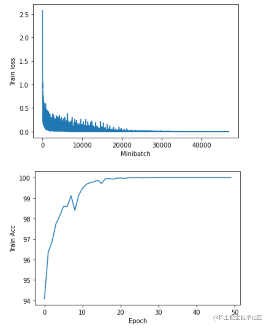
训练过程可视化
import matplotlib
import matplotlib.pyplot as plt
%matplotlib inline

plt.plot(range(len(minibatch_cost)), minibatch_cost)
plt.ylabel('Train loss')
plt.xlabel('Minibatch')
plt.show()

plt.plot(range(len(epoch_acc)), epoch_acc)
plt.ylabel('Train Acc')
plt.xlabel('Epoch')
plt.show()
上述代码☝执行报错,原因是
minibatch_cost的每一个元素都是带有梯度的tensor,无法转化成numpy,解决方法是在此之前添加下面这行代码:minibatch_cost = [a.detach().numpy() for a in minibatch_cost]跑 50 个
epoch的损失和准确率变化图如下👇
- 模型评估
在测试集上的准确率
print('Test accuracy: %.2f%%' % (compute_accuracy(model, test_loader)))结果如下👇
Test accuracy: 98.04%
for features, targets in test_loader:
    break

_, predictions = model.forward(features[:4].view(-1, 28*28))
predictions = torch.argmax(predictions, dim=1)
predictions = predictions.tolist()

fig, ax = plt.subplots(1, 4)
for i in range(4):
    ax[i].imshow(features[i].view(28, 28), cmap=matplotlib.cm.binary)
    ax[i].set_title("Predicted:" + str(predictions[i]))

plt.show()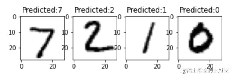
❤️ 感谢大家
感谢大家能看到这里,如果你觉得这篇内容对你有帮助的话:
- 点赞支持下吧,让更多的人也能看到这篇内容。
- 欢迎在留言区与我分享你的想法,也欢迎你在留言区记录你的思考过程。
再次感谢大家的支持与鼓励🌹🌹🌹
ps:此文是本人曾在掘金创作过的文章点此跳转,因此图片带有掘金的水印😅。
评论
登录后参与技术讨论,分享你的经验与见解。
登录 / 注册暂无评论