机器学习还能预测心血管疾病?没错,我用python写出来了

文章目录

CDA数据分析师 出品
作者:Mika
数据:真达
后期:Mika
【导读】手把手教你如何用python写出心血管疾病预测模型。
全球每年约有1700万人死于心血管疾病,当中主要表现为心肌梗死和心力衰竭。当心脏不能泵出足够的血液来满足人体的需要时,就会发生心力衰竭,通常由糖尿病、高血压或其他心脏疾病引起。
在检测心血管疾病的早期症状时,机器学习就能派上用场了。通过患者的电子病历,可以记录患者的症状、身体特征、临床实验室测试值,从而进行生物统计分析,这能够发现那些医生无法检测到的模式和相关性。
尤其通过机器学习,根据数据就能预测患者的存活率,今天我们就教大家如何用Python写一个心血管疾病的预测模型。
研究背景和数据来源
我们用到的数据集来自Davide Chicco和Giuseppe Jurman发表的论文:《机器学习可以仅通过血肌酐和射血分数来预测心力衰竭患者的生存率》。
他们收集整理了299名心力衰竭患者的医疗记录,这些患者数据来自2015年4月至12月间巴基斯坦费萨拉巴德心脏病研究所和费萨拉巴德联合医院。这些患者由105名女性和194名男性组成,年龄在40至95岁之间。所有299例患者均患有左心室收缩功能不全,并曾出现过心力衰竭。
Davide和Giuseppe应用了多个机器学习分类器来预测患者的生存率,并根据最重要的危险因素对特征进行排序。同时还利用传统的生物统计学测试进行了另一种特征排序分析,并将这些结果与机器学习算法提供的结果进行比较。
他们分析对比了心力衰竭患者的一系列数据,最终发现根据血肌酐和射血分数这两项数据能够很好的预测心力衰竭患者的存活率。
今天我们就教教大家,如果根据这共13个字段的299 条病人诊断记录,用Python写出预测心力衰竭患者存活率的预测模型。
下面是具体的步骤和关键代码。
01、数据理解
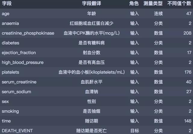
数据取自于kaggle平台分享的心血管疾病数据集,共有13个字段299 条病人诊断记录。具体的字段概要如下:
02、数据读入和初步处理
首先导入所需包。
数据整理
import numpy as np
import pandas as pd
可视化
import matplotlib.pyplot as plt
import seaborn as sns
import plotly as py
import plotly.graph_objs as go
import plotly.express as px
import plotly.figure_factory as ff
模型建立
from sklearn.linear_model import LogisticRegression
from sklearn.tree import DecisionTreeClassifier
from sklearn.ensemble import GradientBoostingClassifier, RandomForestClassifier
import lightgbm
前处理
from sklearn.preprocessing import StandardScaler
模型评估
from sklearn.model_selection import train_test_split, GridSearchCV
from sklearn.metrics import plot_confusion_matrix, confusion_matrix, f1_score
加载并预览数据集:
读入数据
df = pd.read_csv('./data/heart_failure.csv')
df.head()

03、探索性分析
1. 描述性分析
df.describe().T
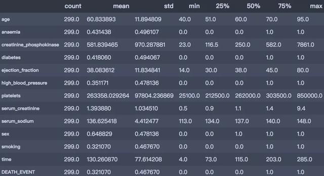
从上述描述性分析结果简单总结如下:
- 是否死亡:平均的死亡率为32%;
- 年龄分布:平均年龄60岁,最小40岁,最大95岁
- 是否有糖尿病:有41.8%患有糖尿病
- 是否有高血压:有35.1%患有高血压
- 是否抽烟:有32.1%有抽烟
2. 目标变量
产生数据
death_num = df['DEATH_EVENT'].value_counts()
death_num = death_num.reset_index()
饼图
fig = px.pie(death_num, names='index', values='DEATH_EVENT')
fig.update_layout(title_text='目标变量DEATH_EVENT的分布')
py.offline.plot(fig, filename='./html/目标变量DEATH_EVENT的分布.html')
总共有299人,其中随访期未存活人数96人,占总人数的32.1%
3. 贫血

从图中可以看出,有贫血症状的患者死亡概率较高,为35.66%。
bar1 = draw_categorical_graph(df['anaemia'], df['DEATH_EVENT'], title='红细胞、血红蛋白减少和是否存活')
bar1.render('./html/红细胞血红蛋白减少和是否存活.html')
4. 年龄
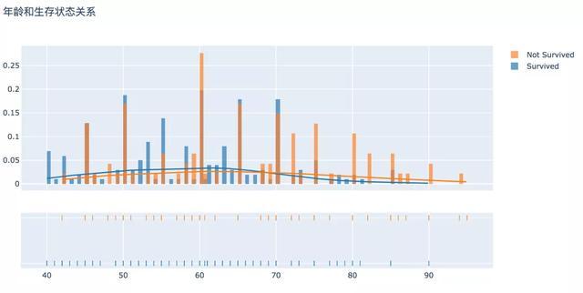
从直方图可以看出,在患心血管疾病的病人中年龄分布差异较大,表现趋势为年龄越大,生存比例越低、死亡的比例越高。
产生数据
surv = df[df['DEATH_EVENT'] == 0]['age']
not_surv = df[df['DEATH_EVENT'] == 1]['age']
hist_data = [surv, not_surv]
group_labels = ['Survived', 'Not Survived']
直方图
fig = ff.create_distplot(hist_data, group_labels, bin_size=0.5)
fig.update_layout(title_text='年龄和生存状态关系')
py.offline.plot(fig, filename='./html/年龄和生存状态关系.html')
5. 年龄/性别
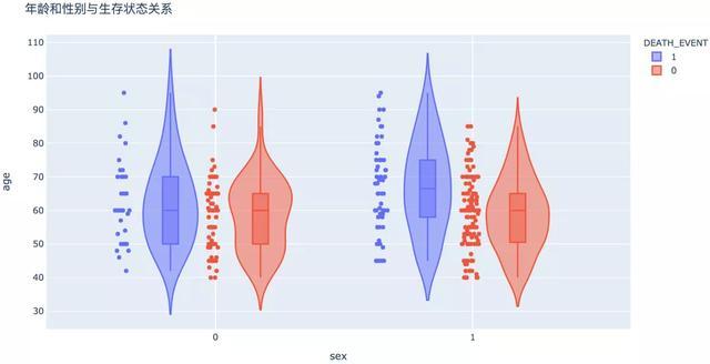
从分组统计和图形可以看出,不同性别之间生存状态没有显著性差异。在死亡的病例中,男性的平均年龄相对较高。
6. 年龄/抽烟
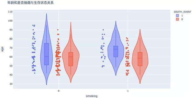
数据显示,整体来看,是否抽烟与生存与否没有显著相关性。但是当我们关注抽烟的人群中,年龄在50岁以下生存概率较高。
7. 磷酸肌酸激酶(CPK)

从直方图可以看出,血液中CPK酶的水平较高的人群死亡的概率较高。
8. 射血分数
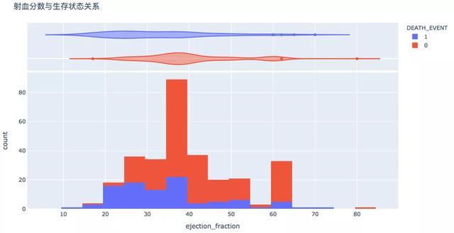
射血分数代表了心脏的泵血功能,过高和过低水平下,生存的概率较低。
9. 血小板
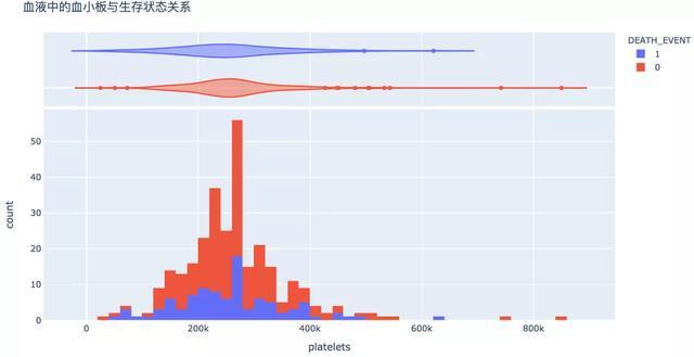
血液中血小板(100~300)×10^9个/L,较高或较低的水平则代表不正常,存活的概率较低。
10. 血肌酐水平

血肌酐是检测肾功能的最常用指标,较高的指数代表肾功能不全、肾衰竭,有较高的概率死亡。
11. 血清钠水平

图形显示,血清钠较高或较低往往伴随着风险。
12. 相关性分析
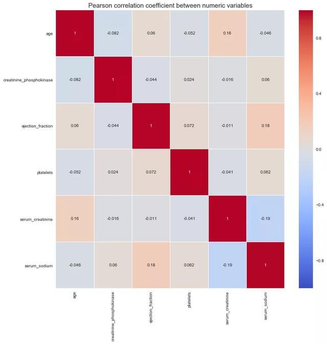
从数值型属性的相关性图可以看出,变量之间没有显著的共线性关系。
num_df = df[['age', 'creatinine_phosphokinase', 'ejection_fraction', 'platelets',
'serum_creatinine', 'serum_sodium']]
plt.figure(figsize=(12, 12))
sns.heatmap(num_df.corr(), vmin=-1, cmap='coolwarm', linewidths=0.1, annot=True)
plt.title('Pearson correlation coefficient between numeric variables', fontdict={'fontsize': 15})
plt.show()
04、特征筛选
我们使用统计方法进行特征筛选,目标变量DEATH_EVENT是分类变量时,当自变量是分类变量,使用卡方鉴定,自变量是数值型变量,使用方差分析。
划分X和y
X = df.drop('DEATH_EVENT', axis=1)
y = df['DEATH_EVENT']
from feature_selection import Feature_select
fs = Feature_select(num_method='anova', cate_method='kf')
X_selected = fs.fit_transform(X, y)
X_selected.head()
2020 17:19:49 INFO attr select success!
After select attr: ['serum_creatinine', 'serum_sodium', 'ejection_fraction', 'age', 'time']

05、数据建模
首先划分训练集和测试集。
划分训练集和测试集
Features = X_selected.columns
X = df[Features]
y = df["DEATH_EVENT"]
X_train, X_test, y_train, y_test = train_test_split(X, y, test_size=0.2, stratify=y,
random_state=2020)
标准化
scaler = StandardScaler()
scaler_Xtrain = scaler.fit_transform(X_train)
scaler_Xtest = scaler.fit_transform(X_test)
lr = LogisticRegression()
lr.fit(scaler_Xtrain, y_train)
test_pred = lr.predict(scaler_Xtest)
F1-score
print("F1_score of LogisticRegression is : ", round(f1_score(y_true=y_test, y_pred=test_pred),2))
我们使用决策树进行建模,设置特征选择标准为gini,树的深度为5。输出混淆矩阵图:在这个案例中,1类是我们关注的对象。
DecisionTreeClassifier
clf = DecisionTreeClassifier(criterion='gini', max_depth=5, random_state=1)
clf.fit(X_train, y_train)
test_pred = clf.predict(X_test)
F1-score
print("F1_score of DecisionTreeClassifier is : ", round(f1_score(y_true=y_test, y_pred=test_pred),2))
绘图
plt.figure(figsize=(10, 7))
plot_confusion_matrix(clf, X_test, y_test, cmap='Blues')
plt.title("DecisionTreeClassifier - Confusion Matrix", fontsize=15)
plt.xticks(range(2), ["Heart Not Failed","Heart Fail"], fontsize=12)
plt.yticks(range(2), ["Heart Not Failed","Heart Fail"], fontsize=12)
plt.show()
F1_score of DecisionTreeClassifier is : 0.61
<Figure size 720x504 with 0 Axes>

使用网格搜索进行参数调优,优化标准为f1。
parameters = {'splitter':('best','random'),
'criterion':("gini","entropy"),
"max_depth":[*range(1, 20)],
}
clf = DecisionTreeClassifier(random_state=1)
GS = GridSearchCV(clf, param_grid=parameters, cv=10, scoring='f1', n_jobs=-1)
GS.fit(X_train, y_train)
print(GS.best_params_)
print(GS.best_score_)
{'criterion': 'entropy', 'max_depth': 3, 'splitter': 'best'}
0.7638956305132776
使用最优的模型重新评估测试集效果:
test_pred = GS.best_estimator_.predict(X_test)
F1-score
print("F1_score of DecisionTreeClassifier is : ", round(f1_score(y_true=y_test, y_pred=test_pred),2))
绘图
plt.figure(figsize=(10, 7))
plot_confusion_matrix(GS, X_test, y_test, cmap='Blues')
plt.title("DecisionTreeClassifier - Confusion Matrix", fontsize=15)
plt.xticks(range(2), ["Heart Not Failed","Heart Fail"], fontsize=12)
plt.yticks(range(2), ["Heart Not Failed","Heart Fail"], fontsize=12)
plt.show()

使用随机森林
RandomForestClassifier
rfc = RandomForestClassifier(n_estimators=1000, random_state=1)
parameters = {'max_depth': np.arange(2, 20, 1) }
GS = GridSearchCV(rfc, param_grid=parameters, cv=10, scoring='f1', n_jobs=-1)
GS.fit(X_train, y_train)
print(GS.best_params_)
print(GS.best_score_)
test_pred = GS.best_estimator_.predict(X_test)
F1-score
print("F1_score of RandomForestClassifier is : ",
round(f1_score(y_true=y_test, y_pred=test_pred),2))
{'max_depth': 3}
0.791157747481277
F1_score of RandomForestClassifier is : 0.53
使用Boosting
gbl = GradientBoostingClassifier(n_estimators=1000, random_state=1)
parameters = {'max_depth': np.arange(2, 20, 1) }
GS = GridSearchCV(gbl, param_grid=parameters, cv=10, scoring='f1', n_jobs=-1)
GS.fit(X_train, y_train)
print(GS.best_params_)
print(GS.best_score_)
测试集
test_pred = GS.best_estimator_.predict(X_test)
F1-score
print("F1_score of GradientBoostingClassifier is : ",
round(f1_score(y_true=y_test, y_pred=test_pred),2))
{'max_depth': 3}
0.7288420428900305
F1_score of GradientBoostingClassifier is : 0.65
使用LGBMClassifier
lgb_clf = lightgbm.LGBMClassifier(boosting_type='gbdt', random_state=1)
parameters = {'max_depth': np.arange(2, 20, 1) }
GS = GridSearchCV(lgb_clf, param_grid=parameters, cv=10, scoring='f1', n_jobs=-1)
GS.fit(X_train, y_train)
print(GS.best_params_)
print(GS.best_score_)
测试集
test_pred = GS.best_estimator_.predict(X_test)
F1-score
print("F1_score of LGBMClassifier is : ", round(f1_score(y_true=y_test, y_pred=test_pred),2))
{'max_depth': 2}
0.780378102289867
F1_score of LGBMClassifier is : 0.74
以下为各模型在测试集上的表现效果对比:
LogisticRegression:0.63
DecisionTree Classifier:0.73
Random Forest Classifier: 0.53
GradientBoosting Classifier: 0.65
LGBM Classifier: 0.74
参考链接:
Machine learning can predict survival of patients with heart failure from serum creatinine and ejection fraction alone
评论
登录后参与技术讨论,分享你的经验与见解。
登录 / 注册暂无评论