逻辑回归

文章目录
Pre learn
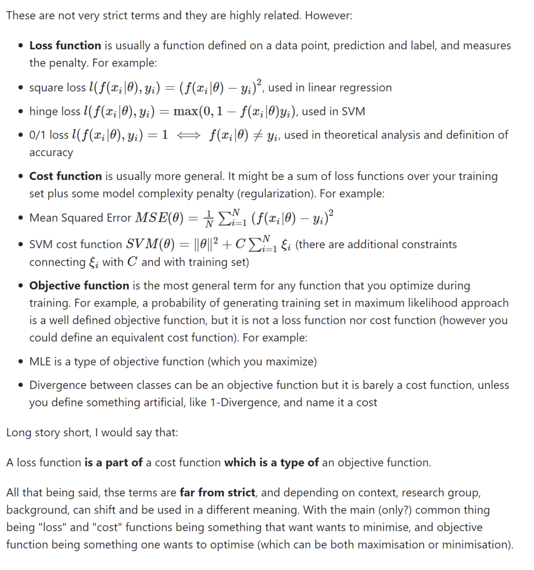
Objective function, cost function, loss function: are they the same thing?
The meaning of theta
\( h(x)=W^TX +b =\theta^Tx\)
Linear regression
Hypotheses:
$$ h_\theta(x)=\theta_0+\theta_1x_1+\theta_2x_2\tag{1} $$
$$ h(x)=\sum_{i=0}^n\theta_ix_i=\theta^Tx\tag{2} $$
$$x_0 =1 $$
Loss:
$$ J(\theta)=\frac 1 2\sum_{i=1}^m(h_\theta(x^{(i)})-y^{(i)})^2\tag{3} $$
式(3)也称Ordinary least squares(最小二乘法),和mean square error(MSE 均方误差)很相似,区别在于:
- 最小二乘法作为损失函数没有除以总样本数m,均方误差除以样本总数m
- 基于均方误差最小化来进行模型求解的方法称为“最小二乘法”。—周志华《机器学习》
至于linear regression loss function为什么是Ordinary least square,详见下方链接pdf里的Probabilistic interpretation.
Goal:
- Ordinary least squares
Solutions:
- Gradient descent
- Normal equation
$$ \theta=(X^TX)^{-1}X^T\vec{y}\tag{4} $$
详见https://see.stanford.edu/materials/aimlcs229/cs229-notes1.pdf
Logistic regression
Logistic function:
$$ g(z)=\frac {1} {1+e^{-z}}\tag{5} $$
$$ g'(z)=g(z)(1-g(z))\tag{6} $$
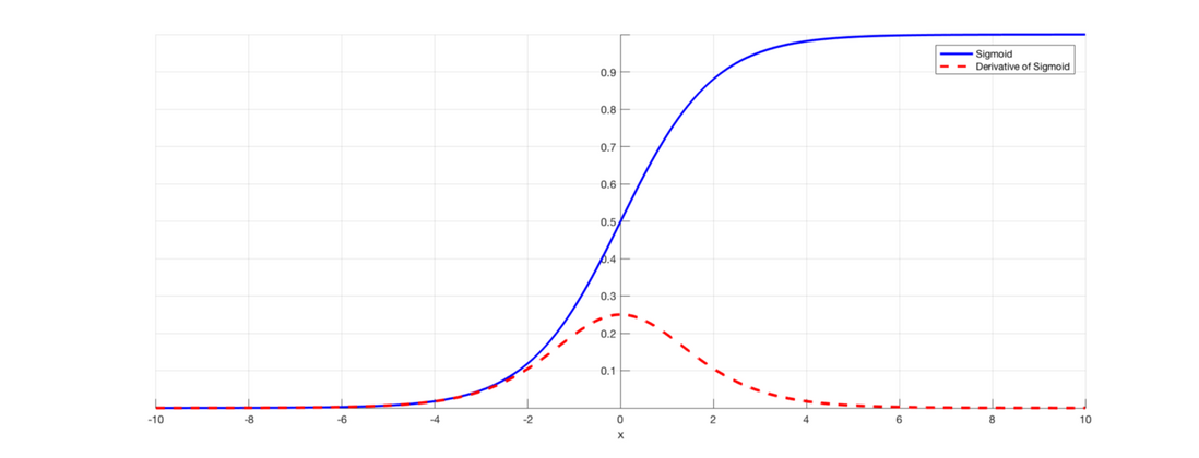
如上图Fig.1所示,sigmoid函数值域为0-1,定义域为R,导数x=0时,其值最大为0.25,但当x趋向于无穷小或无穷大时有梯度消失或梯度爆炸的风险。
Hypotheses:
$$ h_\theta(x)=g(\theta^Tx)=\frac {1} {1+e^{-\theta^Tx}}\tag{7} $$
把线性回归输出输入到逻辑函数里就变成了逻辑回归,值域从R变为0-1,以此就可以作二分类任务,大于0.5是一类,小于0.5是一类。
MLE(Maximum Likelihood Estimate)
接下来从最大似然估计的角度来寻找loss function。
一般by MLE我们想得到argmax p(D\( |\theta) \),即找到参数使得到这样的数据成为可能。
Assume:
$$ P(y=1|x;\theta)=h_\theta(x)\tag{8} $$
$$ P(y=0|x;\theta)=1-h_\theta(x)\tag{9} $$
公式(8)和公式(9)可以合成公式(10):
$$ P(y|x;\theta)=(h_\theta(x))^y(1-h_\theta(x))^{1-y}\tag{10} $$
公式(10)为一个样本的似然概率,也称点估计,那么所以样本的似然概率怎么表示呢?见下式(11):
Likelihood:
$$ \begin{equation}\begin{split} L(\theta)&=p(\vec{y}|X;\theta)\\ &=\prod_{i=1}^{m}p(y^{(i)}|x^{(i)};\theta)\\ &=\prod_{i=1}^{m}(h_\theta(x^{(i)}))^{y^{(i)}}(1-h_\theta(x^{(i)}))^{1-y^{(i)}}\tag{11} \end{split}\end{equation} $$
实际上这就是我们的目标函数,但想找到\( arg\,max{L(\theta)}\)我们还需要进一步简化,简化的方法是前面加一个log,也就是\( log(L(\theta)) \),这样做的好处是:
- 简化方程,将连乘转换成连加
- 防止计算过程中产生数值下溢的风险
- log是单调增函数,不会改变原函数性质
Log Likelihood
$$ \begin{equation}\begin{split} \ell(\theta)&=log(L(\theta))\\ &=\sum_{i=1}^{m}y^{(i)}logh_\theta(x^{(i)})+(1-y^{(i)})log(1-h_\theta(x^{(i)}))\tag{12} \end{split}\end{equation} $$
式(12)就是我们寻找的最大似然函数,其实前面加一个负号就变成了Loss function,只不过最大似然函数追求的是最大值,而Loss function追求的是最小值。
Gradient ascent for one sample:
为了方便求导没有把sum加入计算,也即只针对一个样本
$$ \begin{equation}\begin{split} \frac{\partial \ell(\theta)}{\partial \theta_j}&=(y\frac{1}{g(\theta^Tx)}-(1-y)\frac{1}{1-g(\theta^Tx)})\frac{\partial g(\theta^Tx)}{\theta_j}\\ &=(y\frac{1}{g(\theta^Tx)}-(1-y)\frac{1}{1-g(\theta^Tx)})g(\theta^Tx)(1-g(\theta^Tx))\frac{\partial \theta^Tx}{\theta_j}\\ &=(y(1-g(\theta^Tx))-(1-y)g(\theta^Tx))x_j\\ &=(y-h_\theta(x))x_j\tag{13} \end{split}\end{equation} $$
so, gradient ascent rule:
$$ \theta_j:=\theta_j+\alpha(y^{(i)}-h_\theta(x)^{(i)})x_j^{(i)}\tag{14} $$
Loss function
上面我们提到,式(12)取负号就是我们的loss function:
$$ \arg\,min{-\sum_{i=1}^{m}y^{(i)}logh_\theta(x^{(i)})+(1-y^{(i)})log(1-h_\theta(x^{(i)}))\tag{15}} $$
And gradient descent rule for all samples:
$$ \theta_j:=\theta_j-\alpha\sum_{i=1}^{m}(y^{(i)}-h_\theta(x)^{(i)})x_j^{(i)}\tag{16} $$

As we can see in the figure above, we penalize wrong predictions with an increasingly larger cost.
Regularization:
$$ J(\theta)=-\frac{1}{m}[\sum_{i=1}^{m}y^{(i)}logh_\theta(x^{(i)})+(1-y^{(i)})log(1-h_\theta(x^{(i)}))]+\lambda\sum_{j=1}^m\theta_j^2\tag{17} $$
Gradient descent code
def gradient_descent(X, Y, nx, ny, m, num_iterations, alpha):
    """
    Gradient descent to train parameters.
    """
    W = np.zeros(shape=(nx, 1), dtype=np.float32) # weights initialization
    b = 0.0 # bias initialization
    for i in range(num_iterations):
        Z  = np.dot(W.T, X) + b # shape: (1, m)
        A = sigmoid(Z) # shape: (1, m)

        if i % 1000 == 0:
            # two strategies are both ok
            # mean square error
            cost_1 = -1.0 / m * (np.dot(Y, np.log(A).T) + np.dot((1-Y), np.log(1-A).T))
            print('cost_1:{}'.format(np.squeeze(cost_1)))
            cost_2 = -1.0 / m * np.sum(np.multiply(Y, np.log(A)) + np.multiply(1-Y, np.log(1-A)))
            print('cost_2:{}'.format(cost_2))

        # computation graph
        dZ = A - Y # The derivative of cost to A to Z. shape: (1, m)
        dW = np.dot(X, dZ.T) # The derivative of cost to A to Z to W. shape: (nx, 1)
        W -= 1.0 / m * alpha * dW # update W
        db =  np.sum(dZ) # The derivative of cost to A to Z to b
        b -= 1.0 / m * alpha * db # update b
    return W, b
梯度下降法
梯度下降法的缺点
由式(16)可以看到,我们每更新一次参数都要遍历一次全部样本,而当样本很多的时候,每一次迭代所花费的时间成本是很高的。
随机梯度下降
随机梯度下降法(SGD)可以看作是梯度下降法的极端的情况。在梯度下降法里,每次的参数更新依赖于所有的样本。然而,在随机梯度下降法里,每一次的迭代不再依赖于所有样本的梯度之和,而是仅仅依赖于其中一个样本的梯度。所以这种方法的优势很明显,通过很“便宜”的方式获得梯度,并频繁的对参数做迭代更新,这有助于在更短的时间内得到收敛结果。
gradient descent rule:
$$ \theta_j:=\theta_j-\alpha(y^{(i)}-h_\theta(x)^{(i)})x_j^{(i)}\tag{18} $$
由于在随机梯度下降法中,我们用一个样本的梯度来代替所有样本的梯度之和,计算出来的结果包含大量噪声,并且不太稳定。为了部分解决这个问题,我们通常会把学习率设置为较小的值,这样可以有效削弱梯度计算中带来的不稳定性。
相比梯度下降法,当我们使用随机梯度下降法的时候可以看到每一次迭代之后的目标函数或者损失函数会有一些波动性。有时候的更新会带来目标值的提升,其他时候的更新可能反而让目标值变得更差。但只要实现细节合理,大的趋势是沿着好的方向而发展的。
小批量梯度下降
小批量梯度下降法(mini-batch gradient descent), 它每次从样本中选择一部分子集,并基于这些选出来的样本计算梯度,并做参数的更新。
gradient descent rule:
$$ \theta_j:=\theta_j-\alpha\sum_{i=1}^{n}(y^{(i)}-h_\theta(x)^{(i)})x_j^{(i)}\tag{19} $$
仅选择第1-n个样本,n<m
梯度下降法小结
| 梯度下降法 | 小批量梯度下降法 | 随机梯度下降法 | |
|---|---|---|---|
| 循环样本数 | M(all) | n | 1 |
| 时间复杂度 | O(M) | O(n) | O(1) |
| 稳定性 | 非常强 | 较好 | 弱 |
| 效率 | 慢 | 快 | 快 |
| 实用性 | 弱 | 强 | 较弱 |
在工业界中,最常用的方法为小批量梯度下降法。小批量梯度下降法也有助于更好地利用GPU的计算能力。小批量梯度下降法折中了梯度下降法和随机梯度下降法各自的优缺点,更好地解决梯度噪声的问题,更新更加稳定。
随机梯度下降法或者小批量梯度下降法有助于解决鞍点(saddle point)的问题。
评论
登录后参与技术讨论,分享你的经验与见解。
登录 / 注册暂无评论