ML基础:密度估计基础知识普及!

文章目录
其实密度估计是一个非常简单的概念,我们已经熟悉了一种常见的密度估计技术:直方图。
密度估计在无监督学习,特征工程和数据建模三个领域都有应用。高斯混合模型就是一种流行和有用的密度估计技术和基于近邻域的方法。高斯混合技术还可用作无监督聚类方案。
直方图是一种最简单的数据可视化方法,可以在下图的左上面板中看到:简单的一维核密度估计 这个示例使用sklearn.neighbors。
第一个图显示了使用直方图可视化一维中点密度的问题之一。直观地说,直方图可以被认为是一种方案,其中一个单元“块”被堆放在规则网格的每个点之上。然而,正如最上面的两个面板所显示的,这些块的网格选择可能导致对密度分布的基本形状产生严重分歧。如果我们把每个块放在它所代表的点上,我们就会得到左下角显示的估计值。这个想法可以推广到其他核形状:第一个图的右下角显示了在相同分布上的高斯核密度估计。
Scikit-learn通过sklearn.neighbors使用球树或KD树结构实现有效的核密度估计。KernelDensity估计量。可用的内核显示在本例的第二个图中。
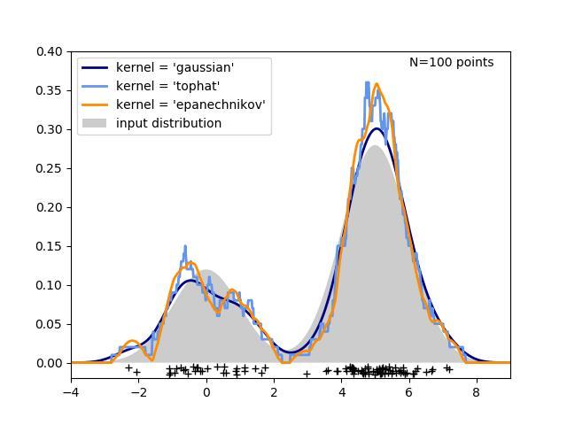
第三个图比较了1维100个样本分布的核密度估计数。虽然本例使用的是一维分布,但核密度估计也可以轻松有效地扩展到更高的维数。

# Author: Jake Vanderplas <jakevdp@cs.washington.edu>
import numpy as np
import matplotlib
import matplotlib.pyplot as plt
from distutils.version import LooseVersion
from scipy.stats import norm
from sklearn.neighbors import KernelDensity
# `normed` is being deprecated in favor of `density` in histograms
if LooseVersion(matplotlib.__version__) >= '2.1':
density_param = {'density': True}
else:
density_param = {'normed': True}
# ----------------------------------------------------------------------
# Plot the progression of histograms to kernels
np.random.seed(1)
N = 20
X = np.concatenate((np.random.normal(0, 1, int(0.3 * N)),
np.random.normal(5, 1, int(0.7 * N))))[:, np.newaxis]
X_plot = np.linspace(-5, 10, 1000)[:, np.newaxis]
bins = np.linspace(-5, 10, 10)
fig, ax = plt.subplots(2, 2, sharex=True, sharey=True)
fig.subplots_adjust(hspace=0.05, wspace=0.05)
# histogram 1
ax[0, 0].hist(X[:, 0], bins=bins, fc='#AAAAFF', **density_param)
ax[0, 0].text(-3.5, 0.31, "Histogram")
# histogram 2
ax[0, 1].hist(X[:, 0], bins=bins + 0.75, fc='#AAAAFF', **density_param)
ax[0, 1].text(-3.5, 0.31, "Histogram, bins shifted")
# tophat KDE
kde = KernelDensity(kernel='tophat', bandwidth=0.75).fit(X)
log_dens = kde.score_samples(X_plot)
ax[1, 0].fill(X_plot[:, 0], np.exp(log_dens), fc='#AAAAFF')
ax[1, 0].text(-3.5, 0.31, "Tophat Kernel Density")
# Gaussian KDE
kde = KernelDensity(kernel='gaussian', bandwidth=0.75).fit(X)
log_dens = kde.score_samples(X_plot)
ax[1, 1].fill(X_plot[:, 0], np.exp(log_dens), fc='#AAAAFF')
ax[1, 1].text(-3.5, 0.31, "Gaussian Kernel Density")
for axi in ax.ravel():
axi.plot(X[:, 0], np.full(X.shape[0], -0.01), '+k')
axi.set_xlim(-4, 9)
axi.set_ylim(-0.02, 0.34)
for axi in ax[:, 0]:
axi.set_ylabel('Normalized Density')
for axi in ax[1, :]:
axi.set_xlabel('x')
# ----------------------------------------------------------------------
# Plot all available kernels
X_plot = np.linspace(-6, 6, 1000)[:, None]
X_src = np.zeros((1, 1))
fig, ax = plt.subplots(2, 3, sharex=True, sharey=True)
fig.subplots_adjust(left=0.05, right=0.95, hspace=0.05, wspace=0.05)
def format_func(x, loc):
if x == 0:
return '0'
elif x == 1:
return 'h'
elif x == -1:
return '-h'
else:
return '%ih' % x
for i, kernel in enumerate(['gaussian', 'tophat', 'epanechnikov',
'exponential', 'linear', 'cosine']):
axi = ax.ravel()[i]
log_dens = KernelDensity(kernel=kernel).fit(X_src).score_samples(X_plot)
axi.fill(X_plot[:, 0], np.exp(log_dens), '-k', fc='#AAAAFF')
axi.text(-2.6, 0.95, kernel)
axi.xaxis.set_major_formatter(plt.FuncFormatter(format_func))
axi.xaxis.set_major_locator(plt.MultipleLocator(1))
axi.yaxis.set_major_locator(plt.NullLocator())
axi.set_ylim(0, 1.05)
axi.set_xlim(-2.9, 2.9)
ax[0, 1].set_title('Available Kernels')
# ----------------------------------------------------------------------
# Plot a 1D density example
N = 100
np.random.seed(1)
X = np.concatenate((np.random.normal(0, 1, int(0.3 * N)),
np.random.normal(5, 1, int(0.7 * N))))[:, np.newaxis]
X_plot = np.linspace(-5, 10, 1000)[:, np.newaxis]
true_dens = (0.3 * norm(0, 1).pdf(X_plot[:, 0])
+ 0.7 * norm(5, 1).pdf(X_plot[:, 0]))
fig, ax = plt.subplots()
ax.fill(X_plot[:, 0], true_dens, fc='black', alpha=0.2,
label='input distribution')
colors = ['navy', 'cornflowerblue', 'darkorange']
kernels = ['gaussian', 'tophat', 'epanechnikov']
lw = 2
for color, kernel in zip(colors, kernels):
kde = KernelDensity(kernel=kernel, bandwidth=0.5).fit(X)
log_dens = kde.score_samples(X_plot)
ax.plot(X_plot[:, 0], np.exp(log_dens), color=color, lw=lw,
linestyle='-', label="kernel = '{0}'".format(kernel))
ax.text(6, 0.38, "N={0} points".format(N))
ax.legend(loc='upper left')
ax.plot(X[:, 0], -0.005 - 0.01 * np.random.random(X.shape[0]), '+k')
ax.set_xlim(-4, 9)
ax.set_ylim(-0.02, 0.4)
plt.show()
下图展示了一个基于地理空间数据的基于邻居的查询示例(特别是核密度估计),使用基于哈弗斯距离度量(即经纬度上的点的距离)构建的球树。如果可以的话,本示例使用basemap绘制南美洲的海岸线和国界。
这个示例没有对数据执行任何学习(请参阅物种分布建模,了解基于此数据集中属性的分类示例)。简单地用地理空间坐标表示观测数据点的核密度估计值。

# Author: Jake Vanderplas <jakevdp@cs.washington.edu>
# License: BSD 3 clause
import numpy as np
import matplotlib.pyplot as plt
from sklearn.datasets import fetch_species_distributions
from sklearn.neighbors import KernelDensity
# if basemap is available, we'll use it.
# otherwise, we'll improvise later...
try:
from mpl_toolkits.basemap import Basemap
basemap = True
except ImportError:
basemap = False
def construct_grids(batch):
"""Construct the map grid from the batch object
Parameters
----------
batch : Batch object
The object returned by :func:`fetch_species_distributions`
Returns
-------
(xgrid, ygrid) : 1-D arrays
The grid corresponding to the values in batch.coverages
"""
# x,y coordinates for corner cells
xmin = batch.x_left_lower_corner + batch.grid_size
xmax = xmin + (batch.Nx * batch.grid_size)
ymin = batch.y_left_lower_corner + batch.grid_size
ymax = ymin + (batch.Ny * batch.grid_size)
# x coordinates of the grid cells
xgrid = np.arange(xmin, xmax, batch.grid_size)
# y coordinates of the grid cells
ygrid = np.arange(ymin, ymax, batch.grid_size)
return (xgrid, ygrid)
# Get matrices/arrays of species IDs and locations
data = fetch_species_distributions()
species_names = ['Bradypus Variegatus', 'Microryzomys Minutus']
Xtrain = np.vstack([data['train']['dd lat'],
data['train']['dd long']]).T
ytrain = np.array([d.decode('ascii').startswith('micro')
for d in data['train']['species']], dtype='int')
Xtrain *= np.pi / 180. # Convert lat/long to radians
# Set up the data grid for the contour plot
xgrid, ygrid = construct_grids(data)
X, Y = np.meshgrid(xgrid[::5], ygrid[::5][::-1])
land_reference = data.coverages[6][::5, ::5]
land_mask = (land_reference > -9999).ravel()
xy = np.vstack([Y.ravel(), X.ravel()]).T
xy = xy[land_mask]
xy *= np.pi / 180.
# Plot map of South America with distributions of each species
fig = plt.figure()
fig.subplots_adjust(left=0.05, right=0.95, wspace=0.05)
for i in range(2):
plt.subplot(1, 2, i + 1)
# construct a kernel density estimate of the distribution
print(" - computing KDE in spherical coordinates")
kde = KernelDensity(bandwidth=0.04, metric='haversine',
kernel='gaussian', algorithm='ball_tree')
kde.fit(Xtrain[ytrain == i])
# evaluate only on the land: -9999 indicates ocean
Z = np.full(land_mask.shape[0], -9999, dtype='int')
Z[land_mask] = np.exp(kde.score_samples(xy))
Z = Z.reshape(X.shape)
# plot contours of the density
levels = np.linspace(0, Z.max(), 25)
plt.contourf(X, Y, Z, levels=levels, cmap=plt.cm.Reds)
if basemap:
print(" - plot coastlines using basemap")
m = Basemap(projection='cyl', llcrnrlat=Y.min(),
urcrnrlat=Y.max(), llcrnrlon=X.min(),
urcrnrlon=X.max(), resolution='c')
m.drawcoastlines()
m.drawcountries()
else:
print(" - plot coastlines from coverage")
plt.contour(X, Y, land_reference,
levels=[-9998], colors="k",
linestyles="solid")
plt.xticks([])
plt.yticks([])
plt.title(species_names[i])
plt.show()
评论
登录后参与技术讨论,分享你的经验与见解。
登录 / 注册暂无评论